Perceptrons
A perceptron classifier is a simple model of a neuron. This machine learning algorithm is used as a supervised learning classifier - a function that given a set of elements can decide if a new element belongs to a predefined category.
The first concept of the perceptron learning rule comes from 1957 Frank Rosenblatt’s paper The Perceptron, a Perceiving and Recognizing Automaton. I can’t recommend reading it highly enough if you are interested in the topic, as Rosenblatt’s explains very clearly the biological similarites of his algorithm proposal.
We can compare the way a Perceptron works as a simple version of a biological neuron: the dentrites recieves signals and the cell body process them. After that processing, the axon’s neuron will send signals out to other neurons.
Now you will think, how does the classifier makes the processing?
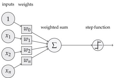
Given an input element, each feature/column is multiplied by a weight value that is assigned to this particular feature. For instance, if the perceptron has a total of five inputs, then five weights will be adjusted for each of these inputs (or features).
All those signals, after multiplied by its weights, will be summed up to a single value. The perceptron also adjusts the offset or bias of those calculations.
^\sum_j w_j x_j + b^
Finally, the result will turn into the output signal. Depending on the sum of the previous calculations an activation function (or transfer function) will classify the result to the category predicted.
We can think about perceptrons as the most basic form of a neural network. The following illustration helps to better to understand the process:
Activation function
The basic form of activation function is the simple binary function that has as a possible results 0 or 1. It basically returns one if the output is positive while zero if it is negative.
-f(s) = ^\begin{cases} 1 & \textrm{if } s \ge 0 \ 0 & \textrm{otherwise} \end{cases}^
Calculate weights and bias of the perceptron
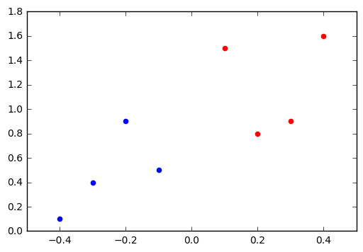
Build the vector of weights is the most tricky and fun part of creating a perceptron. I am going to use Python and a simple set of points to try to illustrate in a simple way how it works – thanks to @fedeisas for guiding me in this process.
| col1 | col2 | target | |
|---|---|---|---|
| 0 | .1 | 1.5 | -1 |
| 1 | .2 | .8 | -1 |
| 2 | .3 | .9 | -1 |
| 3 | .4 | 1.6 | -1 |
| 4 | -.4 | .1 | 1 |
| 5 | -.3 | .4 | 1 |
| 6 | -.2 | .9 | 1 |
| 7 | -.1 | .5 | 1 |
The following code creates our fake training test data with pandas based on the previous table.
import numpy as np
import random
import matplotlib.pyplot as plt
import matplotlib.cm as cm
import pandas as pd

d = {
  'col1': [.1,.2,.3,.4,-.4,-.3,-.2,-.1],
  'col2': [1.5,.8,.9,1.6,.1,.4,.9,.5],
  'target': [-1]*4+[1]*4
}

df = pd.DataFrame(data=d)

pos_mask = df['target'] == 1
neg_mask = df['target'] == -1

plt.scatter(x=df[neg_mask]['col1'], y=df[neg_mask]['col2'], color='r')
plt.scatter(x=df[pos_mask]['col1'], y=df[pos_mask]['col2'], color='b')

plt.show()
The next learning algorithm is the one responsible to train the weights and bias of our perceptron. It initializes all the weights and bias to zero. Then it iterates for all our elements in the training dataset a maxiter number of times, computing the result of the perceptron activation.
For each loop, the function consider that there is an error when the multiplication of the calculated activation and the real output/result is below zero - in other words, it is a wrong prediction. In that case, it updates the weights and bias.
def perceptron_train(max_iter = 10, step = 0.1):
    col_names = df.columns.values[:-1]
    w = dict((name,0) for name in col_names)
    b = 0
    for i in range(max_iter):
        for index, row in df.iterrows():
            a = np.sum([row[col] * w[col] for col in col_names]) + b
            if row['target'] * a <= 0:
                # wrong prediciton
                b += row['target'] * step
                for col in col_names:
                    w[col] += row['target'] * row[col] * step
    return w, b

weights, bias = perceptron_train()
print(weights, bias)
# weights: {'col2': -0.2, 'col1': -0.43}, bias: 0.1
The perceptron training algorithm is considered online, which means that instead of considering and using the entire dataset as a whole, it looks example by example. Once finalized the training of the weights and the bias, the perceptron will be able to make predictions:
def predict(weights, bias, row):
    activation = np.sum([weights[key] * row[key] for key in weights.keys()]) + bias
    return np.sign(activation)
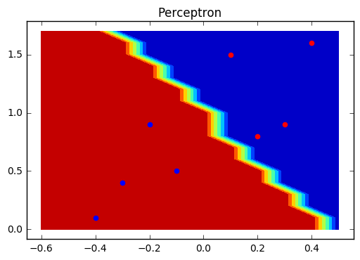
Test our perceptron
A contour plot is a nice way to visually represent the decision boundary of a perceptron. The following code will create the array Z with the predictions of all possible points around our dataset. Calling the function contourf will fill the areas between the values using constant colors corresponding to the current figure’s colormap.
h = .1

# create a meshgrid
x_min, x_max = -0.6, 0.6
y_min, y_max = 0, 1.8
xx, yy = np.meshgrid(np.arange(x_min, x_max, h), np.arange(y_min, y_max, h))

# np.c_ returns a new array with the combination of the ish elem from xx with
# the ish elem of yy
fake = pd.DataFrame(np.c_[xx.ravel(), yy.ravel()], columns=('col1', 'col2'))
Z = np.array([predict(weights, bias, row) for key, row in fake.iterrows()])
# Reshape from array to a matrix of colors
Z = Z.reshape(xx.shape)
fig, ax = plt.subplots()
# contourf(matrix of xs, matrix of ys, and matrix of colors)
ax.contourf(xx, yy, Z)

# Include the training points
# pos_mask = df['target'] == 1
# neg_mask = df['target'] == -1
ax.scatter(x=df[neg_mask]['col1'], y=df[neg_mask]['col2'], color='r')
ax.scatter(x=df[pos_mask]['col1'], y=df[pos_mask]['col2'], color='b')
ax.set_title('Perceptron')
Issues and notes about perceptrons
Notes I have been taken during the research and study of perceptrons - recheck when have some time:
Does the perceptron converge? If so, what does it converge to? And how long does it take? The basic idea of the perceptron is to run a particular algorithm until a linear separator is found. If the data is linearly separable (exists some hyperplane that puts all the positive examples on one side and all the negative examples on the other side) and the learning rate is sufficiently small the perceptron will converge. At some point it will make an entire pass through the training data without making any more updates. On the other hand, if the two classes are not linearly separable the perceptron would never stop updating, that is the reason to set a maximum number of passes.
The perceptron is a linear model that cannot solve the XOR problem.
The perceptron has a lot to gain by feature combination in comparation with decision trees.
Constructing meta features for perceptrons from decision trees: the idea is to train a decision tree on the training data. From that decision tree, you can extract meta features by looking at feature combinations along branches. You can then add only those feature combinations as meta features to the feature set for the perceptron.