Optim In R

December 17, 2016

The function optim in R can be used as an easy way to model the relationship between a dependent value - Y - and one or more independent values - X.

In statistics, linear regression is an approach that studies relationships between continuous (quantitative) variables:

The list of variables, denoted X, is regarded as the predictor, or independent value.
The variable denoted Y, is regarded as the response, or dependent value.

We can define a multiple linear regression with two independent values using optim in R.

Having the dataframe (x, y / z), where (x, y) are the predictors - X - and (z) is the dependent value - Y, we define the linear function ^{z = ax+by+c}^ as our predictive model we are going to optimize.

# our dataframe
> df <- data.frame(x = c(1, 2, 3, 4, 5), y = c(1, 1, 1, 1, 1), z = c(1, 3, 5, 6, 8))
> df
  x y z
1 1 1 1
2 2 1 3
3 3 1 5
4 4 1 6
5 5 1 8

The residual sum of squares (RSS) for our predictive model can be denoted as the following function sumSqMin, where the array par [c, b, a] represents the value for the predictive model z = par[1] + y * par[2] + x * par[3].

This function will be used to fit z against x and y by minimizing the sum of squares. By doing it, it will find the best values a, b and c that we can use in the future to predict new values for z.

sumSqMin <- function(par, data) {
  with(data, sum((par[1] + par[2] * y + par[3] * x - z)^2))
}

Optim minimizes the sum of squares error by varying the parameters par. The first given argument of optim is the array of parameters that will vary, in this case we initialize par as (0, 1, 1); the second argument is the function to be minimized: sumSqMin in this case. Finally, the last argument is our dataframe df.

result <- optim(par = c(0, 1, 1), fn = sumSqMin, data = df)

Let’s print and analyze our result:

> result
$par
[1] -1.3974368  0.8974027  1.7000286

$value
[1] 0.3

$counts
function gradient 
     104       NA 

$convergence
[1] 0

$message
NULL

Our result object includes the parametes par, which provides the best values for c, b and a that minimizes the sum of square errors for the function ^{z = ax+by+c}^.

The parameter value provides the result of calling the function sumSqMin with the previous parameters (-1.3974368, 0.8974027, 1.7000286) and our data frame.

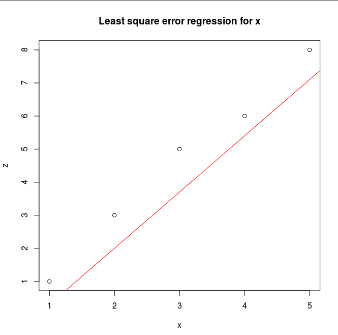
Finally we can plot the result depending on our final parameters, and see if what we have got it is a reasonable prediction (i.e. for our x value):

> plot(z ~ x, data = df, main="Least square error regression for x")
> abline(a = result$par[1], b = result$par[3], col = "red")

alt plot

Back